pandas percentage change

from: https://kanoki.org/2019/09/29/how-to-find-percentage-change-in-pandas/

So you are interested to find the percentage change in your data. Well it is a way to express the change in a variable over the period of time and it is heavily used when you are analyzing or comparing the data. In this post we will see how to calculate the percentage change using pandas pct_change() api and how it can be used with different data sets using its various arguments.
As per the documentation, the definition of pandas pct_change method and its parameters are as shown:

pct_change_(self, periods=1, fill_method=’pad’, limit=None, freq=None,) _
periods : int, default 1 Periods to shift for forming percent change.
fill_method : str, default ‘pad’ How to handle NAs before computing percent changes.
limit : int, default None The number of consecutive NAs to fill before stopping.
freq : DateOffset, timedelta, or offset alias string, optional Increment to use from time series API (e.g. ‘M’ or BDay())

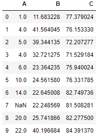
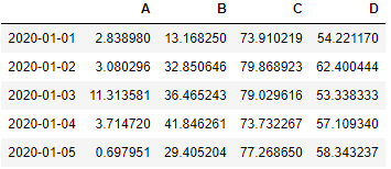
Before we dive deeper into using the pct_change, Lets understand how the Percentage change is calculated across the rows and columns of a dataframe

Create a Dataframe

import pandas as pd
import random
import numpy as np

df = pd.DataFrame({"A":[1,4,5,4,6,10,14,None,20,22],
                   "B":np.random.uniform(low=10.5, high=45.3, size=(10,)),
                   "C":np.random.uniform(low=70.5, high=85, size=(10,))})
df

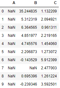
Percentage Change between rows

Here we will find out the percentage change between the rows. We are interested to find out the pct change in value for all indexes across the columns A,B and C. For example: percentage change between Column A and B at index 0 is given by the following formula:

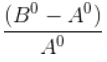
Where B0 is value of column B at index 0 and A0 is value at column A.

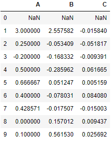
df.pct_change(axis=1)

Percentage Change between two columns

The first row will be NaN since that is the first value for column A, B and C. The percentage change between columns is calculated using the formula:

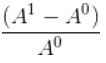
Where A1 is value of column A at index 0 and A1 is value at index 1

df.pct_change(axis=0,fill_method='bfill')

fill_method in pct_change

This is used to fill the NaN values in the data, there are two options i.e. pad and bfill that you can select to fill the NaN values in your data , By default it is pad, which means the NaN values in the data will be filled by the value from preceding row or column whereas bfill which stands for backfill means the NaN values will be filled by the value from succeeding row or column values.
There is another argument limit which is used to decide how many NaN values you want to fill using these methods

Percentage Change for Time series data

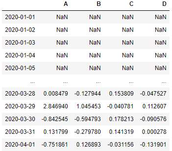
In our time-series data we have the date index with a daily frequency.

import pandas as pd
import random
import numpy as np


# Creating the time-series index
n=92
index = pd.date_range('01/01/2020', periods = n,freq='D')

# Creating the dataframe
df = pd.DataFrame({"A":np.random.uniform(low=0.5, high=13.3, size=(n,)),
                   "B":np.random.uniform(low=10.5, high=45.3, size=(n,)),
                   "C":np.random.uniform(low=70.5, high=85, size=(n,)),
                   "D":np.random.uniform(low=50.5, high=65.7, size=(n,))}, index = index)

df.head()

freq in pct_change()

So using the freq argument you can find the percentage change for any timedelta values, Suppose using this dataframe you want to find out the percentage change after every 5 days then set the freq as 5D. The first five rows is NaN since there are no 5 days back data is present for these values to find the pct change. Only we can start with the 6th row which can be compared with the 1st row to find the pct change for 5 days and similarly we can get pct_change for following rows

df.pct_change(freq='5D')

Monthly pct_change() in time series data

With the same time-series lets find out how to find the monthly pct change in these values. First we need to get the Data for the last day of each month. So we will resample the data for frequency conversion and set the rule as ‘BM’ i.e. Business Month.

monthly = df.resample('BM', how=lambda x: x[-1])

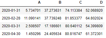
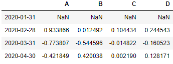
Now apply the pct_change() on this data to find out the monthly percentage change

monthly.pct_change()

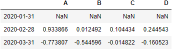
if you want the monthly percentage change for the months which has only the last day date available

df.asfreq('BM').pct_change()

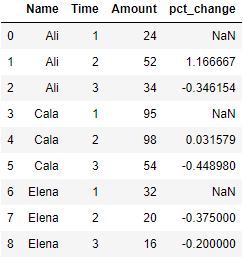
pct_change in groupby

You can also find the percentage change within each group by applying pct_change() on the groupby object. The first value under pct_change() for each group is NaN since we are interested to find the percentage change within each group only.

df = pd.DataFrame({'Name': ['Ali', 'Ali', 'Ali', 'Cala', 'Cala', 'Cala', 'Elena', 'Elena', 'Elena'],
                   'Time': [1, 2, 3, 1, 2, 3, 1, 2, 3],
                   'Amount': [24, 52, 34, 95, 98, 54, 32, 20, 16]})

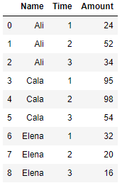
df['pct_change'] = df.groupby(['Name'])['Amount'].pct_change()
df

pandas dataframe axis

AXIS=1

Say if your operation requires traversing from left to right/right to left in a dataframe, you are apparently merging columns ie. you are operating on various columns. This is axis =1

Example

df = pd.DataFrame(np.arange(12).reshape(3,4),columns=['A', 'B', 'C', 'D'])
print(df)
   A  B   C   D
0  0  1   2   3
1  4  5   6   7
2  8  9  10  11 

df.mean(axis=1)

0    1.5
1    5.5
2    9.5
dtype: float64

df.drop(['A','B'],axis=1,inplace=True)

    C   D
0   2   3
1   6   7
2  10  11

 

De actie  die uitgevoerd wordt (bijv MEAN van de kolomwaarde van een rij) gebeurd dus voor iedere rij

AXIS=0

Similarly, if your operation requires traversing from top to bottom/bottom to top in a dataframe, you are merging rows. This is axis=0.

De actie die uitgevoerd wordt, bijv mean (van de rijwaardes van een column)  gebeurt dus voor iedere Column

Pandas Time Series Data Structures

 https://jakevdp.github.io/PythonDataScienceHandbook/03.11-working-with-time-series.html

The fundamental Pandas data structures for working with time series data:

• For time stamps, Pandas provides the Timestamp type. As mentioned before, it is essentially a replacement for Python's native datetime, but is based on the more efficient numpy.datetime64 data type. The associated Index structure is DatetimeIndex.
• For time Periods, Pandas provides the Period type. This encodes a fixed-frequency interval based on numpy.datetime64. The associated index structure is PeriodIndex.
• For time deltas or durations, Pandas provides the Timedelta type. Timedelta is a more efficient replacement for Python's native datetime.timedelta type, and is based on numpy.timedelta64. The associated index structure is TimedeltaIndex.

The most fundamental of these date/time objects are the Timestamp and DatetimeIndex objects. While these class objects can be invoked directly, it is more common to use the pd.to_datetime() function, which can parse a wide variety of formats. Passing a single date to pd.to_datetime() yields a Timestamp; passing a series of dates by default yields a DatetimeIndex:

dates = pd.to_datetime([datetime(2015, 7, 3), '4th of July, 2015',
                       '2015-Jul-6', '07-07-2015', '20150708'])
dates

>DatetimeIndex(['2015-07-03', '2015-07-04', '2015-07-06', '2015-07-07',
               '2015-07-08'],
              dtype='datetime64[ns]', freq=None)

Any DatetimeIndex can be converted to a PeriodIndex with the to_period() function with the addition of a frequency code; here we'll use 'D' to indicate daily frequency:

dates.to_period('D')

PeriodIndex(['2015-07-03', '2015-07-04', '2015-07-06', '2015-07-07',
             '2015-07-08'],
            dtype='int64', freq='D')

A TimedeltaIndex is created, for example, when a date is subtracted from another:

dates - dates[0]

TimedeltaIndex(['0 days', '1 days', '3 days', '4 days', '5 days'], dtype='timedelta64[ns]', freq=None)

 Regular sequences: pd.date_range()

To make the creation of regular date sequences more convenient, Pandas offers a few functions for this purpose:
 pd.date_range() for timestamps,
pd.period_range() for periods, and
pd.timedelta_range() for time deltas.

We've seen that Python's range() and NumPy's np.arange() turn a startpoint, endpoint, and optional stepsize into a sequence. Similarly, pd.date_range() accepts a start date, an end date, and an optional frequency code to create a regular sequence of dates. By default, the frequency is one day:

pd.date_range('2015-07-03', '2015-07-10') 

DatetimeIndex(['2015-07-03', '2015-07-04', '2015-07-05', '2015-07-06',
               '2015-07-07', '2015-07-08', '2015-07-09', '2015-07-10'],
              dtype='datetime64[ns]', freq='D')

Alternatively, the date range can be specified not with a start and endpoint, but with a startpoint and a number of periods:

pd.date_range('2015-07-03', periods=8) 

DatetimeIndex(['2015-07-03', '2015-07-04', '2015-07-05', '2015-07-06',
               '2015-07-07', '2015-07-08', '2015-07-09', '2015-07-10'],
              dtype='datetime64[ns]', freq='D')

The spacing can be modified by altering the freq argument, which defaults to D. For example, here we will construct a range of hourly timestamps:

pd.date_range('2015-07-03', periods=8, freq='H') 

DatetimeIndex(['2015-07-03 00:00:00', '2015-07-03 01:00:00',
               '2015-07-03 02:00:00', '2015-07-03 03:00:00',
               '2015-07-03 04:00:00', '2015-07-03 05:00:00',
               '2015-07-03 06:00:00', '2015-07-03 07:00:00'],
              dtype='datetime64[ns]', freq='H')

To create regular sequences of Period or Timedelta values, the very similar pd.period_range() and pd.timedelta_range() functions are useful. Here are some monthly periods:

pd.period_range('2015-07', periods=8, freq='M') 

PeriodIndex(['2015-07', '2015-08', '2015-09', '2015-10', '2015-11', '2015-12',
             '2016-01', '2016-02'],
            dtype='int64', freq='M')

And a sequence of durations increasing by an hour:

pd.timedelta_range(0, periods=10, freq='H') 

TimedeltaIndex(['00:00:00', '01:00:00', '02:00:00', '03:00:00', '04:00:00',
                '05:00:00', '06:00:00', '07:00:00', '08:00:00', '09:00:00'],
               dtype='timedelta64[ns]', freq='H')

All of these require an understanding of Pandas frequency codes,

Frequencies and Offsets

Fundamental to these Pandas time series tools is the concept of a frequency or date offset. Just as we saw the D (day) and H (hour) codes above, we can use such codes to specify any desired frequency spacing. The following table summarizes the main codes available:

Code	Description	Code	Description
D	Calendar day	B	Business day
W	Weekly
M	Month end	BM	Business month end
Q	Quarter end	BQ	Business quarter end
A	Year end	BA	Business year end
H	Hours	BH	Business hours
T	Minutes
S	Seconds
L	Milliseonds
U	Microseconds
N	nanoseconds

The monthly, quarterly, and annual frequencies are all marked at the end of the specified period. By adding an S suffix to any of these, they instead will be marked at the beginning:

Code	Description		Code	Description
MS	Month start		BMS	Business month start
QS	Quarter start		BQS	Business quarter start
AS	Year start		BAS	Business year start

Additionally, you can change the month used to mark any quarterly or annual code by adding a three-letter month code as a suffix:

• Q-JAN, BQ-FEB, QS-MAR, BQS-APR, etc.
• A-JAN, BA-FEB, AS-MAR, BAS-APR, etc.

In the same way, the split-point of the weekly frequency can be modified by adding a three-letter weekday code:

• W-SUN, W-MON, W-TUE, W-WED, etc.

On top of this, codes can be combined with numbers to specify other frequencies. For example, for a frequency of 2 hours 30 minutes, we can combine the hour (H) and minute (T) codes as follows:

pd.timedelta_range(0, periods=9, freq="2H30T")

TimedeltaIndex(['00:00:00', '02:30:00', '05:00:00', '07:30:00', '10:00:00',
                '12:30:00', '15:00:00', '17:30:00', '20:00:00'],
               dtype='timedelta64[ns]', freq='150T')

All of these short codes refer to specific instances of Pandas time series offsets, which can be found in the pd.tseries.offsets module. For example, we can create a business day offset directly as follows:

from pandas.tseries.offsets import BDay
pd.date_range('2015-07-01', periods=5, freq=BDay())

DatetimeIndex(['2015-07-01', '2015-07-02', '2015-07-03', '2015-07-06',
               '2015-07-07'],
              dtype='datetime64[ns]', freq='B')

For more discussion of the use of frequencies and offsets, see the "DateOffset" section of the Pandas documentation.

Resampling, Shifting, and Windowing

The ability to use dates and times as indices to intuitively organize and access data is an important piece of the Pandas time series tools. The benefits of indexed data in general (automatic alignment during operations, intuitive data slicing and access, etc.) still apply, and Pandas provides several additional time series-specific operations.

resample and asfreq
One common need for time series data is resampling at a higher or lower frequency. This can be done using the resample() method, or the much simpler asfreq() method. The primary difference between the two is that resample() is fundamentally a data aggregation, while asfreq() is fundamentally a data selection.

For up-sampling, resample() and asfreq() are largely equivalent, though resample has many more options available. In this case, the default for both methods is to leave the up-sampled points empty, that is, filled with NA values. Just as with the pd.fillna() function discussed previously, asfreq() accepts a method argument to specify how values are imputed. Here, we will resample the business day data at a daily frequency (i.e., including weekends):

Pandas Time Series: Indexing by Time

Where the Pandas time series tools really become useful is when you begin to index data by timestamps.

For example, we can construct a Series object that has time indexed data:

index = pd.DatetimeIndex(['2014-07-04', '2014-08-04',
                          '2015-07-04', '2015-08-04'])
data = pd.Series([0, 1, 2, 3], index=index)
data

2014-07-04    0
2014-08-04    1
2015-07-04    2
2015-08-04    3
dtype: int64

Now that we have this data in a Series, we can make use of any of the Series indexing patterns we discussed in previous sections, passing values that can be coerced into dates:

data['2014-07-04':'2015-07-04']

2014-07-04    0
2014-08-04    1
2015-07-04    2
dtype: int64

There are additional special date-only indexing operations, such as passing a year to obtain a slice of all data from that year:

data['2015']

2015-07-04    2
2015-08-04    3
dtype: int64

date and time python

date en time data voorkomens

• Time stamps reference particular moments in time (e.g., July 4th, 2015 at 7:00am).
• Time intervals and periods reference a length of time between a particular beginning and end point; for example, the year 2015. Periods usually reference a special case of time intervals in which each interval is of uniform length and does not overlap (e.g., 24 hour-long periods comprising days).
• Time deltas or durations reference an exact length of time (e.g., a duration of 22.56 seconds).

DATE AND TIMES IN PYTHON

Er zijn verschillende packages in python mbt times, dates , deltas

native python dates en times: packages Datetime and dateutil

handig voor veel zaken zoals het opbouwen van datetime, dates en conversies.

niet handig als when you wish to work with large arrays of dates and times: just as lists of Python numerical variables are suboptimal compared to NumPy-style typed numerical arrays, lists of Python datetime objects are suboptimal compared to typed arrays of encoded dates.

typed arrays of times: NumPy's datetime64

The weaknesses of Python's datetime format inspired the NumPy team to add a set of 

native time series data type to NumPy. The datetime64 dtype encodes dates as 64-bit integers, 

and thus allows arrays of dates to be represented very compactly.

One detail of the datetime64 and timedelta64 objects is that they are built on a 

fundamental time unit. Because the datetime64 object is limited to 64-bit precision, 

the range of encodable times is 264 times this fundamental unit. In other words, 

datetime64 imposes a trade-off between time resolution and maximum time span. 

 Anderd nadeel dat het niet zo handig werkt als datetime and dateutil

Pandas dates and times Beste alternatief

Pandas builds upon all the tools just discussed to provide a Timestamp object, which combines the ease-of-use of datetime and dateutil with the efficient storage and vectorized interface of numpy.datetime64. From a group of these Timestamp objects, Pandas can construct a DatetimeIndex that can be used to index data in a Series or DataFrame; we'll see many examples of this below.

For example, we can use Pandas tools to repeat the demonstration from above. We can parse a flexibly formatted string date, and use format codes to output the day of the week:

import pandas as pd
date = pd.to_datetime("4th of July, 2015")
date 

>Timestamp('2015-07-04 00:00:00')

date.strftime('%A')

>'Saturday'

Additionally, we can do NumPy-style vectorized operations directly on this same object:

date + pd.to_timedelta(np.arange(12), 'D')

>DatetimeIndex(['2015-07-04', '2015-07-05', '2015-07-06', '2015-07-07',
               '2015-07-08', '2015-07-09', '2015-07-10', '2015-07-11',
               '2015-07-12', '2015-07-13', '2015-07-14', '2015-07-15'],
              dtype='datetime64[ns]', freq=None)

else if in lambda functions

how to use else if in lambda functions

f = lambda x: 1 if x>0 else 0 if x ==0 else -1

dfGert.apply(lambda x: 1 if pd.isnull(x['EIND_DATUM']) else 2 , axis=1  ) 

dfGert['TEST']= dfGert.apply(lambda x: x['Dossier afsluitdatum'] if x['EIND_DATUM'] > x['Dossier afsluitdatum'] else x['EIND_DATUM'] , axis=1  )

miniconda anaconda configuratie

-hoe activeer je environment in een Anaconda prompt

activate  O:\Input\03_ZichtenGrip\python\environments\ENV_flask_dash

let op UNC  paden

\\swappams2820.basis.lan\IVS_BI_Ontwikkel\data\Input\03_ZichtenGrip\python\environments\ENV_flask_dash

- Hoe wordt anaconda prompt aangeroepen

call "%windir%\System32\cmd.exe "/K" C:\Users\wagene002\AppData\Local\Continuum\miniconda3\Scripts\activate.bat C:\Users\wagene002\AppData\Local\Continuum\miniconda3"

- Hoe wordt anaconda prompt aangeroepen met eigen Environment (startConda Environment.bat)

echo "hi"
call "%windir%\System32\cmd.exe "/K"  C:\Users\wagene002\AppData\Local\Continuum\miniconda3\Scripts\activate.bat O:\Input\03_ZichtenGrip\python\environments\ENV_flask_dash\
C:\Users\wagene002\Desktop\runit.bat
echo "bye"


For Windows, use the following script in your batch file to execute a Python script. Simply change your personal file paths.

cmd /c C:\ProgramData\Anaconda3\condabin\conda.bat run "C:\ProgramData\Anaconda3\python.exe" "C:\Users\User Name\Path to your Python File\Python File.py"

hoe start je een python script

cmd /c C:\Users\wagene002\AppData\Local\Continuum\miniconda3\condabin\conda.bat run "\\swappams2820.basis.lan\IVS_BI_Ontwikkel\data\Input\03_ZichtenGrip\python\environments\ENV_flask_dash\python.exe" "\\swappams2820.basis.lan\IVS_BI_Ontwikkel\data\Input\03_ZichtenGrip\python\scripts\CheckStagingWMON.py"

hoe start je de juiste miniconda omgeving en geef je daarna het juiste python commanda

call "%windir%\System32\cmd.exe "/K"  C:\Users\wagene002\AppData\Local\Continuum\miniconda3\Scripts\activate.bat O:\Input\03_ZichtenGrip\python\environments\ENV_flask_dash\  & cmd /c C:\Users\wagene002\AppData\Local\Continuum\miniconda3\condabin\conda.bat run "\\swappams2820.basis.lan\IVS_BI_Ontwikkel\data\Input\03_ZichtenGrip\python\environments\ENV_flask_dash\python.exe" "\\swappams2820.basis.lan\IVS_BI_Ontwikkel\data\Input\03_ZichtenGrip\python\scripts\CheckStagingWMON.py"

let op de essentie zit hem in eerst de shel starten van miniconda en daarna na de & het commando geven

conda offline installation

conda install <package-file-name>.tar.bz2

 C:\Users\wagene002\Desktop>conda install O:\Input\03_ZichtenGrip\pandas-datareader-0.8.1-py_0.tar.bz2

Vergelijken dataframes

Vergelijken van 2 dataframes met elkaaar


def VergelijkTabellen(dfBase,dfCurrent) :
    dfC=pd.merge(dfBase,dfCurrent, on='table_name', how='outer',suffixes=('_old', '_new'))
#    Analyses
    logger.info('------------------------------' + str(datetime.now()) + '------------------------------' )
  
    logger.info('tabellen alleen in old' )
    t=dfC[(dfC['aantal_old'].isna() &  dfC['aantal_new'].notna())]
    logger.info(t.to_string(columns=['table_name'],index=False))
    logger.info('------------------------------')
    logger.info('tabellen alleen in new' )
    t=dfC[(dfC['aantal_old'].notna() &  dfC['aantal_new'].isna())]
    logger.info(t.to_string(columns=['table_name'],index=False))
    t=dfC[(dfC['aantal_old'].notna() &  dfC['aantal_new'].notna())]
    dfC['Verschil']=dfC.apply(lambda x : x['aantal_new'] - x['aantal_old'], axis=1)
  
    lstValues=[(dfC['aantal_new'] - dfC['aantal_old']) /(dfC['aantal_old'])]
    lstConditions = [dfC['aantal_old'].notna() & dfC['aantal_new'].notna() & dfC['aantal_old']!=0 ]
    dfC['Stijging']= np.select(lstConditions,lstValues,'nvt')
    dfC['Stijging'] = dfC['Stijging'].map(lambda x : '{percent:.2%}'.format(percent=float(x)) if x!= 'nvt' else x)
  
    logger.info(dfC.to_string(index=False))
    return dfC

Percentages printen van strings.

    dfC['Stijging'] = dfC['Stijging'].map(lambda x : '{percent:.2%}'.format(percent=float(x)))

Percentage berekenen

     lstValues=[(dfC['aantal_new'] - dfC['aantal_old']) /(dfC['aantal_old'])]
    lstConditions = [dfC['aantal_old'].notna() & dfC['aantal_new'].notna() & dfC['aantal_old']!=0 ]
    dfC['Stijging']= np.select(lstConditions,lstValues,'nvt')

    dfC['Stijging'] = dfC['Stijging'].map(lambda x : '{percent:.2%}'.format(percent=float(x)) if x!= 'nvt' else x)

Create pandas columns based on multiple conditions

Create columns based on other values in the row

 df1['Verschil']=df1.apply(lambda x : x['aantal_new'] - x['aantal_old'], axis=1)

Create pandas columns based on multiple conditions

With pandas and numpy we barely have to write our own functions, especially since our own functions will perform slow because these are not vectorized and pandas + numpy provide a rich pool of vectorized methods for us.

In this case your are looking for np.select since you want to create a column based on multiple conditions:

definieer 2 lijsten van dezelfde lengte
1 lijst met de where clauses
1 lijst met de values


lstValues=[(df1['aantal_new'] - df1['aantal_old']) /(df1['aantal_old']),'99999999999']

lstConditions = [df1['aantal_old'].notna() & df1['aantal_new'].notna(), df1['aantal_old'].isna() &  
df1['aantal_new'].isna()]
 
df1['Stijging2']= np.select(lstConditions,lstValues,'99')

How to iterate over rows in a DataFrame in Pandas?

How to iterate over rows in a DataFrame in Pandas?


Iterating through pandas objects is generally slow. In many cases, iterating manually over the rows is not needed [...].

Answer: DON'T!

Iteration in pandas is an anti-pattern, and is something you should only do when you have exhausted every other option. You should not use any function with "iter" in its name for more than a few thousand rows or you will have to get used to a lot of waiting.
Do you want to print a DataFrame? Use DataFrame.to_string().
Do you want to compute something? In that case, search for methods in this order (list modified from here):

1. Vectorization
2. Cython routines
3. List Comprehensions (vanilla for loop)
4. DataFrame.apply(): i)  Reductions that can be performed in cython, ii) Iteration in python space
5. DataFrame.itertuples() and iteritems()
6. DataFrame.iterrows()

iterrows and itertuples (both receiving many votes in answers to this question) should be used in very rare circumstances, such as generating row objects/nametuples for sequential processing, which is really the only thing these functions are useful for.

Faster than Looping: Vectorization, Cython

A good number of basic operations and computations are "vectorised" by pandas (either through NumPy, or through Cythonized functions). This includes arithmetic, comparisons, (most) reductions, reshaping (such as pivoting), joins, and groupby operations. Look through the documentation on Essential Basic Functionality to find a suitable vectorised method for your problem.
If none exists, feel free to write your own using custom cython extensions.

---

Next Best Thing: List Comprehensions

List comprehensions should be your next port of call if 1) there is no vectorized solution available, 2) performance is important, but not important enough to go through the hassle of cythonizing your code, and 3) you're trying to perform elementwise transformation on your code. There is a good amount of evidence to suggest that list comprehensions are sufficiently fast (and even sometimes faster) for many common pandas tasks.
The formula is simple,

# iterating over one column - `f` is some function that processes your data
result = [f(x) for x in df['col']]
# iterating over two columns, use `zip`
result = [f(x, y) for x, y in zip(df['col1'], df['col2'])]
# iterating over multiple columns
result = [f(row[0], ..., row[n]) for row in df[['col1', ...,'coln']].values]

If you can encapsulate your business logic into a function, you can use a list comprehension that calls it. You can make arbitrarily complex things work through the simplicity and speed of raw python.

logging

Voorbeeld mbt  logging gebruiken:

"""
voorbeeld van een loghandler die output wegschrijft naar een file.
gebruikt een log handler en overschrijft de file. Wel na herstart spyder anders schrijft ie bij
"""
import logging



logger = logging.getLogger(__name__) 
 
# set log level
logger.setLevel(logging.INFO)
 
# define file handler and set formatter. Overwrite logfile w+
file_handler = logging.FileHandler(r'C:\Users\wagene002\Documents\Python\grip\vergelijkinglZenG\\testlog.log','w+')
 
#formatter    = logging.Formatter('%(asctime)s : %(levelname)s : %(name)s : %(message)s')
formatter    = logging.Formatter()
file_handler.setFormatter(formatter)
logger.addHandler(file_handler)
 

#logging.basicConfig(level=logging.INFO, filename='vergelijkBIster_datamodel.log',filemode='w')

logger.info('Er heeft een verandering plaatsgevonden mbt de volgende tabellen: ')




links
https://www.loggly.com/ultimate-guide/python-logging-basics/
https://tutorialedge.net/python/python-logging-best-practices/
https://realpython.com/python-logging/

BSN valid

# maakt gebruik van stdnum module;   conda install -c hargup/label/pypi python-stdnum
import numpy as np
import pandas as pd
import os
from stdnum.nl import bsn
#------INITIALISATI

def BSN_is_valid(tbsn):
    from stdnum.nl import bsn   
    if bsn.is_valid(tbsn) :
        return 1
    else:
        return 0